We are excited to be part of the Robust Vision Challenge 2020. Check out the challenge website and our submission instructions for further details
On this page, we describe our acquisition setup and the processing pipeline to generate reference data with uncertainties for stereo and optical flow. More details are given in the video and our publications [2] and [5].
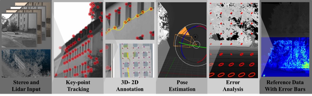
Our approach is divided into the following steps:
The resulting error distributions of the inputs (LIDAR, image data, intrinsics) and derived inputs (extrinsics) are mapped into image space and, subsequently, into disparity space using both analytic error propagation and Monte Carlo sampling.
Once the trajectory of the camera is obtained for a sequence, the trajectories of sequences with similar illumination are found automatically. Here the 2d-3D correspondence estimation problem is reduced to a 2D-2D problem by using the intensity images of the first sequence as a proxy (see [5] for details).
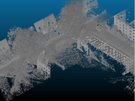
A reference 3D point cloud was collected using a Mobile Mapping System RIEGL VMX-250-CS6, which was equipped with two calibrated laser scanners RIEGL VQ-250 and four cameras. During data collection, position and orientation is determined using the integrated Applanix POS-LV 510 system, consisting of a high-precision global navigation satellite system (GNSS) receiver, an inertial measurement unit (IMU), and an odometer.
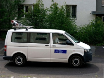
The first processing step computes a post-processed trajectory from GNSS, IMU, odometer and external GNSS base station data (Applanix software). In the second step, the georeferenced 3D point cloud is obtained from this trajectory and the recorded raw laser scanner data (RIEGL software).
The measurement accuracy and precision of the laser scanners is 10 mm and 5 mm, respectively (both 1σ). Absolute accuracy of the point cloud mainly depends on IMU and GNSS performance. Under perfect conditions - no GNSS outages, post-processing with GNSS base station and odometer enabled - an absolute position accuracy of 2 to 5 cm is achievable. Under adverse conditions, especially in built-up areas, GNSS outages and multi-path effects may lead to a lower absolute accuracy, typically in the range of 15-30 cm in height and 20 cm in position. Nevertheless, the relative (local) accuracy of the points along one scan is usually much better, in the range of a few centimeters.
Each laser scanner provides a 360® profile range measurement, at 100 profiles per second and 300 kHz measurement rate. This leads to a point pattern on the ground with a spacing of 2 mm per meter distance across track and 1 cm per m/s vehicle speed along track. For example, at 10 m/s (36 km/h) forward movement of the mobile mapping van, points on a facade in 50 m distance will approximately form a regularly spaced, 10 cm x 10 cm grid.
Due to online waveform processing, multiple targets can be detected with each laser beam. This leads to a good penetrability through non-solid obstacles, such as bushes, trees or fences. However, if two objects are too close, it will be impossible to separate the echoes, and mixed points may result.
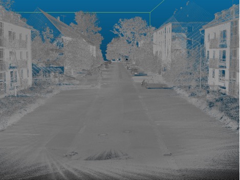
For easier handling of the data, the point cloud is projected to UTM coordinates (using EPSG code 25832) and sorted into a regular grid of 25 m times 25 m cell size. In addition to 3D coordinates (East, North, altitude), timestamp and reflectance information is included for every point. 8.4 million points.
The stereo system used in this project consists of two pco.edge 5.5 cameras with parallel mounted optical axes. The baseline of 30 cm is oriented in x-direction. The sensor of each camera has the dimensions of 14.04 mm x 16.64 mm at a resolution of 2160x 2560 with a pixel pitch of 6.5 µm. With a rolling shutter and at this resolution the maximal bandwidth of the used cameralink interface limits the frame rate to 100 Hz.
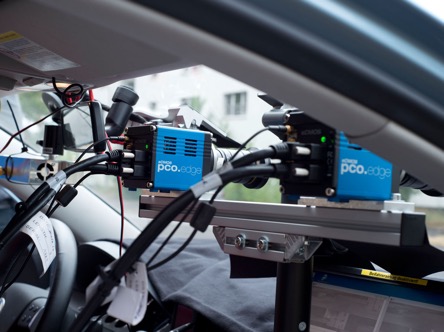
We used a configuration with a resolution of 1080 x 2560, so we could achieve a maximal frame rate of almost 200 Hz. These cameras have a dynamic range of 27000:1 linearly encoded in 16 bit values, which were mapped to 8 bit values through a non-linear noise equilibrating transform without a loss of information [4]. Each camera was connected to the system through a Silicon Software microEnable IV VD4-CL Framegrabber card, which supports the Camera Link Full standard and custom on-board image processing through a programmable FPGA.
Two Kowa LM12XC C-Mount lenses with a focal length of 12 mm (horizontal FoV: 69®) were used at f-Numbers ranging from 2 to 8, depending on the light conditions. The exposure time was adjusted to avoid saturation in the images and ranged from 0.5 to 4.9 ms.
Due to the high data rate of the cameras, it was not possible to record directly to disk. So the limiting resource for the maximal length of a sequence was the available memory, which in our case was 128 GB. This corresponds to a maximal continuous recording time of 100 s, where after the data had to be written to disk.
We determined the internal camera parameters of the stereo camera pair using the method described by Abraham and Hau. The RMS reprojection error reached 0.22 pixel with a variance of 3.6 pixel. We also measured lens distortions and performed all subsequent calculations on the undistorted and stereo rectified images.
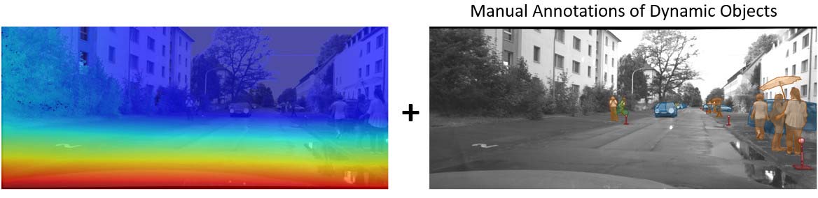
No known measurement technique exists to directly estimate dense flow or depth for dynamic objects. To fill in the missing data in these areas, we used a card boarding scheme as follows: Dynamic objects in the reference dataset where manually segmented using Pallas Ludens technology. The static reference depth or optical flow at these dynamic regions is ignored for this benchmark. We describe in [3] how performance evaluation can still be performed at these regions with cardboarding and specific evaluation metrics.